L’échéance approche à grands pas pour s’inscrire à un atelier lors du prochain ISVEE14 qui aura lieu à Merida, Mexique (31 juillet). Il y a un choix de plusieurs ateliers, tous aussi intéressants les uns que les autres, mais visant souvent un public qui a déjà une certaine expérience en épidémiologie et analyse de données. Cependant beaucoup de chercheurs ne sont pas familiers aux meilleures pratiques et outils requis dans le cycle de vie des données, de la gestion de ces données, la saisie et la création de métadonnées, l’analyse des données, à leur partage et leur ré-utilisation.
Data Carpentry vise à apprendre ces compétences qui permettent aux chercheurs d’être plus efficaces et productifs. Un atelier de 3 jours est proposé après la conférence ISVEE (8, 9 et 10 novembre).
Cet atelier est conçu pour les personnes avec peu ou pas d’expérience informatique (càd public novice), procurant les concepts de base, les compétences et outils pour travailler de manière plus efficace avec des données. Notre méthode d’enseignement est pratique, les participants doivent donc apporter leur propre ordinateur portable. Nous fournirons à l’avance les instructions nécessaires pour installer les logiciels requis et de l’aide sera disponible sur place. Aucun pré-requis n’est demandé et les outils utilisés ne requièrent pas de connaissances préalables. Aucune connaissance particulière en statistiques n’est demandée. Les chercheurs à différents niveaux dans leur carrière sont ciblés (étudiants au doctorat, chercheurs post-doctoraux, chercheurs associés, dans l’industrie ou au gouvernement, …). Le programme comprend:
comment utiliser des tableurs (tels que Excel) plus efficacement, et leurs limites,
passer de ces tableurs à des outils plus puissants pour manipuler et analyser les données, avec le logiciel statistique R,
se servir de bases de données, incluant les gérer et interroger avec SQL,
utiliser Git, un système de contrôle de version de pointe qui permet de suivre qui fait des changements à quoi et quand,
établir un flux de travail et automatiser les tâches répétitives, en particulier en ayant recours à la ligne de commande shell et aux scripts shell.
Les instructeurs ont appris beaucoup de ces compétences à leurs dépens et savent la différence qu’elles peuvent apporter à leur productivité et la possibilité de nouvelles ou meilleures recherches qu’elles permettent.
La recherche reproductible est importante et de bonnes pratiques sont essentielles.
On se revoit à Merida!
Plus d’informations à propos de l’atelier Data Carpentry à ISVEE ici.
Last post on modelling survival data from Veterinary Epidemiologic Research: parametric analyses. The Cox proportional hazards model described in the last post make no assumption about the shape of the baseline hazard, which is an advantage if you have no idea about what that shape might be. With a parametric survival model, the survival time is assumed to follow a known distribution: Weibull, exponential (which is a special case of the Weibull), log-logistic, log-normal, and generalized gamma.
Exponential Model
The exponential model is the simplest, the hazard is constant over time: the rate at which failures are occurring is constant, . We use again the pgtrial dataset:
Interpretation is the same as for a Cox model. Exponentiated coefficients are hazard ratios. R outputs the parameter estimates of the AFT (accelerated failure time) form of the exponential model. If you multiply the estimated coefficients by minus one you get estimates that are consistent with the proportional hazards parameterization of the model. So for tx, the estimated hazard ratio is exp(0.2178) = 1.24 (at any given point in time, a treated cow is 1.24 times more likely to conceive than a non-treated cow). The corresponding accelerating factor for an exponential model is the reciprocal of the hazard ratio, exp(-0.2178) = 0.80: treating a cow accelerates the time to conception by a factor of 0.80.
Weibull Model
In a Weibull model, the hazard function is where and are > 0. is the shape parameter and determines the shape of the hazard function. If it’s , the hazard increases with time. If , the hazard is constant and the model reduces to an exponential model. If , the hazard decreases over time.
The shape parameter is the reciprocal of what is called by R the scale parameter. The shape parameter is then 1/1.15 = 0.869.
We can also use a piecewise constant exponential regression model, which is a model allowing the baseline hazard to vary between time periods but forces it to remain constant within time periods. In order to run such a model, we need data in a counting process format with a start and stop time for each interval. However, survreg does not allow for a data in that format. The trick would be to use a glm and fitting a Poisson model, including time intervals. See this post by Stephanie Kovalchik which explains how to construct the data and model. The example below is using the same approach, for a time interval of 40 days:
interval.width <- 40
# function to compute time breaks given the exit time = dar
cow.breaks <- function(dar) unique(c(seq(0, dar, by = interval.width),
                                      dar))
# list of each subject's time periods
the.breaks <- lapply(unique(pgtrial$cow), function(id){
  cow.breaks(max(pgtrial$dar[pgtrial$cow == id]))
})
# the expanded period of observation:
start <- lapply(the.breaks, function(x) x[-length(x)]) # for left time points
stop <-  lapply(the.breaks, function(x) x[-1]) # for right time points

count.per.cow <- sapply(start, length)
index <- tapply(pgtrial$cow, pgtrial$cow, length)
index <- cumsum(index) # index of last observation for each cow

event <- rep(0, sum(count.per.cow))
event[cumsum(count.per.cow)] <- pgtrial$preg[index]

# creating the expanded dataset
pw.pgtrial <- data.frame(
    cow = rep(pgtrial$cow[index], count.per.cow),
    dar = rep(pgtrial$dar[index], count.per.cow),
    herd = rep(pgtrial$herd[index], count.per.cow),
    tx = rep(pgtrial$tx[index], count.per.cow),
    lact = rep(pgtrial$lact[index], count.per.cow),
    thin = rep(pgtrial$thin[index], count.per.cow),
    start = unlist(start),
    stop = unlist(stop),
    event = event
  )

# create time variable which indicates the period of observation (offset in Poisson model)
pw.pgtrial$time <- pw.pgtrial$stop - pw.pgtrial$start # length of observation

# create a factor for each interval, allowing to have a different rate for each period
pw.pgtrial$interval <- factor(pw.pgtrial$start)

pw.pgtrial[100:110, ]
    cow dar herd tx lact   thin start stop event time interval
100  61 113    1  1    4   thin     0   40     0   40        0
101  61 113    1  1    4   thin    40   80     0   40       40
102  61 113    1  1    4   thin    80  113     1   33       80
103  62 117    1  0    7 normal     0   40     0   40        0
104  62 117    1  0    7 normal    40   80     0   40       40
105  62 117    1  0    7 normal    80  117     2   37       80
106  63 121    1  1    1   thin     0   40     0   40        0
107  63 121    1  1    1   thin    40   80     0   40       40
108  63 121    1  1    1   thin    80  120     0   40       80
109  63 121    1  1    1   thin   120  121     2    1      120
110  64 122    1  1    3 normal     0   40     0   40        0

# Poisson model
pw.model <- glm(event ~ offset(log(time)) + interval + herd + tx + lact +
+                 thin, data = pw.pgtrial, family = "poisson")
summary(pw.model)

Call:
glm(formula = event ~ offset(log(time)) + interval + herd + tx +
    lact + thin, family = "poisson", data = pw.pgtrial)

Deviance Residuals:
   Min      1Q  Median      3Q     Max
-1.858  -1.373  -1.227   1.357   3.904

Coefficients:
             Estimate Std. Error z value Pr(>|z|)
(Intercept) -3.602545   0.132436 -27.202  < 2e-16 ***
interval40  -0.112838   0.106807  -1.056  0.29076
interval80  -0.064105   0.125396  -0.511  0.60920
interval120 -0.007682   0.147919  -0.052  0.95858
interval160 -0.005743   0.191778  -0.030  0.97611
interval200 -0.427775   0.309143  -1.384  0.16644
interval240  0.199904   0.297331   0.672  0.50137
interval280  0.737508   0.385648   1.912  0.05583 .
interval320  0.622366   1.006559   0.618  0.53637
herd2       -0.254389   0.114467  -2.222  0.02626 *
herd3        0.026851   0.119416   0.225  0.82209
tx           0.219584   0.084824   2.589  0.00963 **
lact        -0.023528   0.027511  -0.855  0.39241
thinthin    -0.139915   0.093632  -1.494  0.13509
---
Signif. codes:  0 ‘***’ 0.001 ‘**’ 0.01 ‘*’ 0.05 ‘.’ 0.1 ‘ ’ 1

(Dispersion parameter for poisson family taken to be 1)

    Null deviance: 2155.6  on 798  degrees of freedom
Residual deviance: 2131.1  on 785  degrees of freedom
AIC: 2959.1

Number of Fisher Scoring iterations: 7
Individual Frailty Model
In an individual frailty model, we add variance unique to individuals in order to account for additional variability in the hazard (like negative binomial model vs. Poisson model). For example, let’s fit a Weibull model with gamma individual frailty to the prostaglandin dataset:
Shared Frailty
Shared frailty is a way to deal with clustered data. We will use the “culling” dataset and fit a shared frailty model with a Weibull distribution and a gamma distributed frailty common to all cows in a herd:
Next on modelling survival data from Veterinary Epidemiologic Research: semi-parametric analyses. With non-parametric analyses, we could only evaluate the effect one or a small number of variables. To evaluate multiple explanatory variables, we analyze data with a proportional hazards model, the Cox regression. The functional form of the baseline hazard is not specified, which make the Cox model a semi-parametric model.
A Cox proportional hazards model is fit hereafter, on data from a clinical trial of the effect of prostaglandin adminsitration on the start of breeding period of dairy cows:
R gives several options to control ties in case several events occurred at the same time: the Efron method (default in R), Breslow method (default in software like SAS or Stata), and the exact method. Breslow is the simplest and adequate if not too many ties in the dataset. Efron is closer to the exact approximation.
Stratified Cox Propotional Hazards Model
In a stratified Cox model, different baseline hazards are assumed across groups of subjects. The Cox model is modified to allow the control of a predictor which do not satisfy the proportional hazards (PH) assumption. We refit the above model by stratifying by herd and including a treatment by herd interaction:
scoxph.mod <- coxph(Surv(dar, preg == 'pregnant') ~ tx + tx*herd + lact + thin +
                    strata(herd), data = pgtrial, method = 'breslow')
summary(scoxph.mod)
Call:
coxph(formula = Surv(dar, preg == "pregnant") ~ tx + tx * herd +
    lact + thin + strata(herd), data = pgtrial, method = "breslow")

  n= 319, number of events= 264

             coef exp(coef) se(coef)      z Pr(>|z|)
tx       -0.02160   0.97863  0.25528 -0.085   0.9326
herd2          NA        NA  0.00000     NA       NA
herd3          NA        NA  0.00000     NA       NA
lact     -0.04600   0.95504  0.04065 -1.132   0.2578
thinthin -0.13593   0.87291  0.13833 -0.983   0.3258
tx:herd2 -0.05659   0.94498  0.33570 -0.169   0.8661
tx:herd3  0.54494   1.72451  0.31823  1.712   0.0868 .
---
Signif. codes:  0 ‘***’ 0.001 ‘**’ 0.01 ‘*’ 0.05 ‘.’ 0.1 ‘ ’ 1

         exp(coef) exp(-coef) lower .95 upper .95
tx          0.9786     1.0218    0.5934     1.614
herd2           NA         NA        NA        NA
herd3           NA         NA        NA        NA
lact        0.9550     1.0471    0.8819     1.034
thinthin    0.8729     1.1456    0.6656     1.145
tx:herd2    0.9450     1.0582    0.4894     1.825
tx:herd3    1.7245     0.5799    0.9242     3.218

Concordance= 0.56  (se = 0.035 )
Rsquare= 0.032   (max possible= 0.998 )
Likelihood ratio test= 10.32  on 5 df,   p=0.06658
Wald test            = 10.5  on 5 df,   p=0.0623
Score (logrank) test = 10.66  on 5 df,   p=0.05851
Evaluating the Assumption of Proportional Hazards
We can evaluate it graphically, by examining the log-cumulative hazard plot vs. ln(time) and check if the curves are parallel:
Another graphical approach is to compare plots of predicted survival times from a Cox model (assuming PH) to Kaplan-Meier survivor function (which do not assume PH):
You can also assess PH statistically with the Schoenfeld residuals using cox.zph function:
(schoen <- cox.zph(coxph.mod))
             rho chisq      p
herd2    -0.0630 1.100 0.2942
herd3    -0.0443 0.569 0.4506
tx       -0.1078 3.141 0.0763
lact      0.0377 0.447 0.5035
thinthin -0.0844 2.012 0.1560
GLOBAL        NA 7.631 0.1778

plot(schoen, var = 4)
Schoenfeld residuals for lactation
Evaluating the Overall Fit of the Model
First we can look at the Cox-Snell residuals, which are the estimated cumulative hazards for individuals at their failure (or censoring) times. The default residuals of coxph in R are the martingale residuals, not the Cox-Snell. But it can be computed:
## GOF (Gronnesby and Borgan omnibus gof)
library(gof)
cumres(coxph.mod)

Kolmogorov-Smirnov-test: p-value=0.35
Cramer von Mises-test: p-value=0.506
Based on 1000 realizations. Cumulated residuals ordered by herd2-variable.
---
Kolmogorov-Smirnov-test: p-value=0.041
Cramer von Mises-test: p-value=0.589
Based on 1000 realizations. Cumulated residuals ordered by herd3-variable.
---
Kolmogorov-Smirnov-test: p-value=0
Cramer von Mises-test: p-value=0.071
Based on 1000 realizations. Cumulated residuals ordered by tx-variable.
---
Kolmogorov-Smirnov-test: p-value=0.728
Cramer von Mises-test: p-value=0.733
Based on 1000 realizations. Cumulated residuals ordered by lact-variable.
---
Kolmogorov-Smirnov-test: p-value=0.106
Cramer von Mises-test: p-value=0.091
Based on 1000 realizations. Cumulated residuals ordered by thinthin-variable.
We can evaluate the concordance between the predicted and observed sequence of pairs of events. Harrell’s c index computes the proportion of all pairs of subjects in which the model correctly predicts the sequence of events. It ranges from 0 to 1 with 0.5 for random predictions and 1 for a perfectly discriminating model. It is obtained from the Somer’s Dxy rank correlation:
library(rms)
fit.cph <- cph(Surv(dar, preg == 'pregnant') ~ herd + tx + lact + thin,
               data = pgtrial, x = TRUE, y = TRUE, surv = TRUE)
v <- validate(fit.cph, dxy = TRUE, B = 100)
Dxy <- v[rownames(v) == "Dxy", colnames(v) == "index.corrected"]
(Dxy / 2) + 0.5 # c index
[1] 0.4538712
Evaluating the Functional Form of Predictors
We can use martingale residuals to evaluate the functional form of the relationship between a continuous predictor and the survival expectation for individuals:
lact.mod <- coxph(Surv(dar, preg == 'pregnant') ~ lact, data = pgtrial,
                  ties = 'breslow')
lact.res <- resid(lact.mod, type = "martingale")
plot(pgtrial$lact, lact.res, xlab = 'lactation', ylab = 'Martingale residuals')
lines(lowess(pgtrial$lact, lact.res, iter = 0))

# adding quadratic term
lact.mod <- update(lact.mod, . ~ . + I(lact^2))
lact.res <- resid(lact.mod, type = "martingale")
plot(pgtrial$lact, lact.res, xlab = 'lactation', ylab = 'Martingale residuals')
lines(lowess(pgtrial$lact, lact.res, iter = 0))
Plot of marrtingale residuals vs. lactation numberPlot of martingale residuals vs. lactation number (as quadratic term)
Checking for Outliers
Deviance residuals can be used to identify outliers:
Next topic from Veterinary Epidemiologic Research: chapter 19, modelling survival data. We start with non-parametric analyses where we make no assumptions about either the distribution of survival times or the functional form of the relationship between a predictor and survival. There are 3 non-parametric methods to describe time-to-event data: actuarial life tables, Kaplan-Meier method, and Nelson-Aalen method.
We use data on occurrence of calf pneumonia in calves raised in 2 different housing systems. Calves surviving to 150 days without pneumonia are considered censored at that time.
To create a life table, we use the function lifetab from package KMsurv, after calculating the number of censored and events at each time point and grouping them by time interval (with gsummary from package nlme).
To compute the Kaplan-Meier estimator we use the function survfit from package survival. It takes as argument a Surv object, which gives the time variable and the event of interest. You get the Kaplan-Meier estimate with the summary of the survfit object. We can then plot the estimates to show the Kaplan-Meier survivor function.
A “hazard” is the probability of failure at a point in time, given that the calf had survived up to that point in time. A cumulative hazard, the Nelson-Aaalen estimate, can be computed. The Nelson-Aalen estimate can be calculated by transforming the Fleming-Harrington estimate of survival.
Several tests are available to test whether the overall survivor functions in 2 or more groups are equal. We can use the log-rank test, the simplest test, assigning equal weight to each time point estimate and equivalent to a standard Mantel-Haenszel test. Also, there’s the Peto-Peto-Prentice test which weights the stratum-specific estimates by the overall survival experience and so reduces the influence of different censoring patterns between groups.
To do these tests, we apply the survdiff function to the Surv object. The argument rho gives the weights according to and may be any numeric value. Default is rho = 0 which gives the log-rank test. Rho = 1 gives the “Peto & Peto modification of the Gehan-Wilcoxon test”. Rho larger than zero gives greater weight to the first part of the survival curves. Rho smaller than zero gives weight to the later part of the survival curves.
survdiff(Surv(days, pn == 1) ~ stock, data = calf_pneu, rho = 0) # rho is optional
Call:
survdiff(formula = Surv(days, pn == 1) ~ stock, data = calf_pneu,
    rho = 0)

                  N Observed Expected (O-E)^2/E (O-E)^2/V
stock=batch      12        4     6.89      1.21      2.99
stock=continuous 12        8     5.11      1.63      2.99

 Chisq= 3  on 1 degrees of freedom, p= 0.084

survdiff(Surv(days, pn == 1) ~ stock, data = calf_pneu, rho = 1) # rho=1 asks for Peto-Peto test
Call:
survdiff(formula = Surv(days, pn == 1) ~ stock, data = calf_pneu,
    rho = 1)

                  N Observed Expected (O-E)^2/E (O-E)^2/V
stock=batch      12     2.89     5.25      1.06      3.13
stock=continuous 12     6.41     4.05      1.38      3.13

 Chisq= 3.1  on 1 degrees of freedom, p= 0.0766
Finally we can compare survivor function with stock R plot or using ggplot2. With ggplot2, you get the necessary data from the survfit object and create a new data frame from it. The baseline data (time = 0) are not there so you create it yourself:
As noted on paragraph 18.4.1 of the book Veterinary Epidemiologic Research, logistic regression is widely used for binary data, with the estimates reported as odds ratios (OR). If it’s appropriate for case-control studies, risk ratios (RR) are preferred for cohort studies as RR provides estimates of probabilities directly. Moreover, it is often forgotten the assumption of rare event rate, and the OR will overestimate the true effect.
One approach to get RR is to fit a generalised linear model (GLM) with a binomial distribution and a log link. But these models may sometimes fail to converge (Zou, 2004). Another option is to use a Poisson regression with no exposure or offset specified (McNutt, 2003). It gives estimates with very little bias but confidence intervals that are too wide. However, using robust standard errors gives correct confidence intervals (Greenland, 2004, Zou, 2004).
We use data on culling of dairy cows to demonstrate this.
Continuing on the examples from the book Veterinary Epidemiologic Research, we look today at modelling count when the count of zeros may be higher or lower than expected from a Poisson or negative binomial distribution. When there’s an excess of zero counts, you can fit either a zero-inflated model or a hurdle model. If zero counts are not possible, a zero-truncated model can be use.
Zero-inflated models
Zero-inflated models manage an excess of zero counts by simultaneously fitting a binary model and a Poisson (or negative binomial) model. In R, you can fit zero-inflated models (and hurdle models) with the library pscl. We use the fec dataset which give the fecal egg counts of gastro-intestinal nematodes from 313 cows in 38 dairy herds where half of the observations have zero counts. The predictors in the model are lactation (primiparous vs. multiparous), access to pasture, manure spread on heifer pasture, and manure spread on cow pasture.
We can assess if the zero-inflated model fits the data better than a Poisson or negative binomial model with a Vuong test. If the value of the test is 1.96 indicates superiority of model 1 over model 2. If the value lies between -1.96 and 1.96, neither model is preferred.
### fit same model with negative binomial
library(MASS)
mod3.nb <- glm.nb(fec ~ lact + past_lact + man_heif + man_lact, data = fec)
### Vuong test
vuong(mod3, mod3.nb)
Vuong Non-Nested Hypothesis Test-Statistic: 3.308663
(test-statistic is asymptotically distributed N(0,1) under the
 null that the models are indistinguishible)
in this case:
model1 > model2, with p-value 0.0004687128

### alpha
1/mod3$theta
[1] 3.895448
The Vuong statistic is 3.3 (p < 0.001) indicating the first model, the zero-inflated one, is superior to the regular negative binomial. Note that R does not estimate but its inverse, . is 3.9, suggesting a negative binomial is preferable to a Poisson model.
The parameter modelled in the binary part is the probability of a zero count: having lactating cows on pasture reduced the probability of a zero count ( = -1.8), and increased the expected count if it was non-zero ( = 0.54).
Hurdle models
A hurdle model has also 2 components but it is based on the assumption that zero counts arise from only one process and non-zero counts are determined by a different process. The odds of non-zero count vs. a zero count is modelled by a binomial model while the distribution of non-zero counts is modelled by a zero-truncated model. We refit the fec dataset above with a negative binomial hurdle model:
mod4 <- hurdle(fec ~ lact + past_lact + man_heif + man_lact, data = fec, dist = "negbin")
summary(mod4)

Call:
hurdle(formula = fec ~ lact + past_lact + man_heif + man_lact, data = fec,
    dist = "negbin")

Pearson residuals:
    Min      1Q  Median      3Q     Max
-0.4598 -0.3914 -0.3130 -0.1479 23.6774

Count model coefficients (truncated negbin with log link):
            Estimate Std. Error z value Pr(>|z|)
(Intercept)   1.1790     0.4801   2.456  0.01407 *
lact         -1.1349     0.1386  -8.187 2.69e-16 ***
past_lact     0.5813     0.1782   3.261  0.00111 **
man_heif     -0.9854     0.1832  -5.379 7.50e-08 ***
man_lact      1.0139     0.1998   5.075 3.87e-07 ***
Log(theta)   -2.9111     0.5239  -5.556 2.76e-08 ***
Zero hurdle model coefficients (binomial with logit link):
            Estimate Std. Error z value Pr(>|z|)
(Intercept) -0.13078    0.10434  -1.253  0.21006
lact        -0.84485    0.09728  -8.684  < 2e-16 ***
past_lact    0.84113    0.11326   7.427 1.11e-13 ***
man_heif    -0.35576    0.13582  -2.619  0.00881 **
man_lact     0.85947    0.15337   5.604 2.10e-08 ***
---
Signif. codes:  0 '***' 0.001 '**' 0.01 '*' 0.05 '.' 0.1 ' ' 1

Theta: count = 0.0544
Number of iterations in BFGS optimization: 25
Log-likelihood: -5211 on 11 Df
We can compare zero-inflated and hurdle models by their log-likelihood. The hurdle model fits better:
logLik(mod4)
'log Lik.' -5211.18 (df=11)
logLik(mod3)
'log Lik.' -5238.622 (df=11)
### Null model for model 3:
mod3.null <- update(mod3, . ~ 1)
logLik(mod3.null)
'log Lik.' -5428.732 (df=3)
Zero-truncated model
Sometimes zero counts are not possible. In a zero-truncated model, the probability of a zero count is computed from a Poisson (or negative binomial) distribution and this value is subtracted from 1. The remaining probabilities are rescaled based on this difference so they total 1. We use the daisy2 dataset and look at the number of services required for conception (which cannot be zero…) with the predictors parity, days from calving to first service, and presence/absence of vaginal discharge.
temp <- tempfile()
download.file(
  "http://ic.upei.ca/ver/sites/ic.upei.ca.ver/files/ver2_data_R.zip", temp)
load(unz(temp, "ver2_data_R/daisy2.rdata"))
unlink(temp)

library(VGAM)
mod5 <- vglm(spc ~ parity + cf + vag_disch, family = posnegbinomial(), data = daisy2)
summary(mod5)

Call:
vglm(formula = spc ~ parity + cf + vag_disch, family = posnegbinomial(),
    data = daisy2)

Pearson Residuals:
               Min       1Q    Median      3Q    Max
log(munb)  -1.1055 -0.90954  0.071527 0.82039 3.5591
log(size) -17.4891 -0.39674 -0.260103 0.82155 1.4480

Coefficients:
                Estimate Std. Error z value
(Intercept):1  0.1243178 0.08161432  1.5232
(Intercept):2 -0.4348170 0.10003096 -4.3468
parity         0.0497743 0.01213893  4.1004
cf            -0.0040649 0.00068602 -5.9254
vag_disch      0.4704433 0.10888570  4.3205

Number of linear predictors:  2

Names of linear predictors: log(munb), log(size)

Dispersion Parameter for posnegbinomial family:   1

Log-likelihood: -10217.68 on 13731 degrees of freedom

Number of iterations: 5
As cows get older, the number of services required increase, and the longer the first service was delayed, the fewer services were required.
The first intercept is the usual intercept. The second intercept is the over dispersion parameter .
Still going through the book Veterinary Epidemiologic Research and today it’s chapter 18, modelling count and rate data. I’ll have a look at Poisson and negative binomial regressions in R.
We use count regression when the outcome we are measuring is a count of number of times an event occurs in an individual or group of individuals. We will use a dataset holding information on outbreaks of tuberculosis in dairy and beef cattle, cervids and bison in Canada between 1985 and 1994.
temp <- tempfile()
download.file(
"http://ic.upei.ca/ver/sites/ic.upei.ca.ver/files/ver2_data_R.zip",
temp)
load(unz(temp, "ver2_data_R/tb_real.rdata"))
unlink(temp)

library(Hmisc)
tb_real<- upData(tb_real, labels = c(farm_id = 'Farm identification',
                            type = 'Type of animal',
                            sex = 'Sex', age = 'Age category',
                            reactors = 'Number of pos/reactors in the group',
                            par = 'Animal days at risk in the group'),
                 levels = list(type = list('Dairy' = 1, 'Beef' = 2,
                                 'Cervid' = 3, 'Other' = 4),
                   sex = list('Female' = 0, 'Male' = 1),
                   age = list('0-12 mo' = 0, '12-24 mo' = 1, '>24 mo' = 2)))
An histogram of the count of TB reactors is shown hereafter:
hist(tb_real$reactors, breaks = 0:30 - 0.5)
In a Poisson regression, the mean and variance are equal.
A Poisson regression model with type of animal, sex and age as predictors, and the time at risk is:
mod1 <- glm(reactors ~ type + sex + age + offset(log(par)), family = poisson, data = tb_real)
(mod1.sum <- summary(mod1))

Call:
glm(formula = reactors ~ type + sex + age + offset(log(par)),
    family = poisson, data = tb_real)

Deviance Residuals:
    Min       1Q   Median       3Q      Max
-3.5386  -0.8607  -0.3364  -0.0429   8.7903

Coefficients:
            Estimate Std. Error z value Pr(>|z|)
(Intercept) -11.6899     0.7398 -15.802  < 2e-16 ***
typeBeef      0.4422     0.2364   1.871 0.061410 .
typeCervid    1.0662     0.2334   4.569 4.91e-06 ***
typeOther     0.4384     0.6149   0.713 0.475898
sexMale      -0.3619     0.1954  -1.852 0.064020 .
age12-24 mo   2.6734     0.7217   3.704 0.000212 ***
age>24 mo     2.6012     0.7136   3.645 0.000267 ***
---
Signif. codes:  0 ‘***’ 0.001 ‘**’ 0.01 ‘*’ 0.05 ‘.’ 0.1 ‘ ’ 1

(Dispersion parameter for poisson family taken to be 1)

    Null deviance: 409.03  on 133  degrees of freedom
Residual deviance: 348.35  on 127  degrees of freedom
AIC: 491.32

Number of Fisher Scoring iterations: 8

### here's an other way of writing the offset in the formula:
mod1b <- glm(reactors ~ type + sex + age, offset = log(par), family = poisson, data = tb_real)
Quickly checking the overdispersion, the residual deviance should be equal to the residual degrees of freedom if the Poisson errors assumption is met. We have 348.4 on 127 degrees of freedom. The overdispersion present is due to the clustering of animals within herd, which was not taken into account.
The incidence rate and confidence interval can be obtained with:
cbind(exp(coef(mod1)), exp(confint(mod1)))
Waiting for profiling to be done...
                                2.5 %       97.5 %
(Intercept) 8.378225e-06 1.337987e-06 2.827146e-05
typeBeef    1.556151e+00 9.923864e-01 2.517873e+00
typeCervid  2.904441e+00 1.866320e+00 4.677376e+00
typeOther   1.550202e+00 3.670397e-01 4.459753e+00
sexMale     6.963636e-01 4.687998e-01 1.010750e+00
age12-24 mo 1.448939e+01 4.494706e+00 8.867766e+01
age>24 mo   1.347980e+01 4.284489e+00 8.171187e+01
As said in the post for logistic regression, the profile likelihood-based CI is preferable due to the Hauck-Donner effect (overestimation of the SE) (see also abstract by H. Stryhn at ISVEE X).
The deviance and Pearson goodness-of-fit test statistics can be done with:
Diagnostics can be obtained as usual (see previous posts) but we can also use the Anscombe residuals:
library(wle)
mod1.ansc <- residualsAnscombe(tb_real$reactors, mod1$fitted.values, family = poisson())

plot(predict(mod1, type = "response"), mod1.ansc)
plot(cooks.distance(mod1), mod1.ansc)
Diagnostic plot – Anscombe residuals vs. predicted counts Diagnostic plot – Anscombe residuals vs. Cook’s distance
Negative binomial regression models are for count data for which the variance is not constrained to equal the mean. We can refit the above model as a negative binomial model using full maximum likelihood estimation:
library(MASS)
mod2 <- glm.nb(reactors ~ type + sex + age + offset(log(par)), data = tb_real)
(mod2.sum <- summary(mod2))

Call:
glm.nb(formula = reactors ~ type + sex + age + offset(log(par)),
    data = tb_real, init.theta = 0.5745887328, link = log)

Deviance Residuals:
     Min        1Q    Median        3Q       Max
-1.77667  -0.74441  -0.45509  -0.09632   2.70012

Coefficients:
             Estimate Std. Error z value Pr(>|z|)
(Intercept) -11.18145    0.92302 -12.114  < 2e-16 ***
typeBeef      0.60461    0.62282   0.971 0.331665
typeCervid    0.66572    0.63176   1.054 0.291993
typeOther     0.80003    0.96988   0.825 0.409442
sexMale      -0.05748    0.38337  -0.150 0.880819
age12-24 mo   2.25304    0.77915   2.892 0.003832 **
age>24 mo     2.48095    0.75283   3.296 0.000982 ***
---
Signif. codes:  0 ‘***’ 0.001 ‘**’ 0.01 ‘*’ 0.05 ‘.’ 0.1 ‘ ’ 1

(Dispersion parameter for Negative Binomial(0.5746) family taken to be 1)

    Null deviance: 111.33  on 133  degrees of freedom
Residual deviance:  99.36  on 127  degrees of freedom
AIC: 331.47

Number of Fisher Scoring iterations: 1


              Theta:  0.575
          Std. Err.:  0.143

 2 x log-likelihood:  -315.472

### to use a specific value for the link parameter (2 for example):
mod2b <- glm(reactors ~ type + sex + age + offset(log(par)),
             family = negative.binomial(2), data = tb_real)
Next topic on logistic regression: the exact and the conditional logistic regressions.
Exact logistic regression
When the dataset is very small or severely unbalanced, maximum likelihood estimates of coefficients may be biased. An alternative is to use exact logistic regression, available in R with the elrm package. Its syntax is based on an events/trials formulation. The dataset has to be collapsed into a data frame with unique combinations of predictors.
Another possibility is to use robust standard errors, and get comparable p-values to those obtained with exact logistic regression.
### exact logistic regression
x <- xtabs(~ casecont + interaction(dneo, dclox), data = nocardia)
x
        interaction(dneo, dclox)
casecont 0.0 1.0 0.1 1.1
       0  20  15   9  10
       1   2  44   3   5
> nocardia.coll <- data.frame(dneo = rep(1:0, 2), dclox = rep(1:0, each = 2),
+                    casecont = x[1, ], ntrials = colSums(x))
nocardia.coll
    dneo dclox casecont ntrials
0.0    1     1       20      22
1.0    0     1       15      59
0.1    1     0        9      12
1.1    0     0       10      15

library(elrm)
Le chargement a nécessité le package : coda
Le chargement a nécessité le package : lattice
mod5 <- elrm(formula = casecont/ntrials ~ dneo,
             interest = ~dneo,
             iter = 100000, dataset = nocardia.coll, burnIn = 2000)

### robust SE
library(robust)
Le chargement a nécessité le package : fit.models
Le chargement a nécessité le package : MASS
Le chargement a nécessité le package : robustbase
Le chargement a nécessité le package : rrcov
Le chargement a nécessité le package : pcaPP
Le chargement a nécessité le package : mvtnorm
Scalable Robust Estimators with High Breakdown Point (version 1.3-02)

mod6 <- glmrob(casecont ~ dcpct + dneo + dclox + dneo*dclox,
+                family = binomial, data = nocardia, method= "Mqle",
+                control= glmrobMqle.control(tcc=1.2))
> summary(mod6)

Call:  glmrob(formula = casecont ~ dcpct + dneo + dclox + dneo * dclox,      family = binomial, data = nocardia, method = "Mqle", control = glmrobMqle.control(tcc = 1.2))


Coefficients:
             Estimate Std. Error z-value Pr(>|z|)
(Intercept) -4.440253   1.239138  -3.583 0.000339 ***
dcpct        0.025947   0.008504   3.051 0.002279 **
dneo         3.604941   1.034714   3.484 0.000494 ***
dclox        0.713411   1.193426   0.598 0.549984
dneo:dclox  -2.935345   1.367212  -2.147 0.031797 *
---
Signif. codes:  0 ‘***’ 0.001 ‘**’ 0.01 ‘*’ 0.05 ‘.’ 0.1 ‘ ’ 1
Robustness weights w.r * w.x:
 89 weights are ~= 1. The remaining 19 ones are summarized as
   Min. 1st Qu.  Median    Mean 3rd Qu.    Max.
 0.1484  0.4979  0.6813  0.6558  0.8764  0.9525

Number of observations: 108
Fitted by method ‘Mqle’  (in 5 iterations)

(Dispersion parameter for binomial family taken to be 1)

No deviance values available
Algorithmic parameters:
   acc    tcc
0.0001 1.2000
maxit
   50
test.acc
  "coef"
Conditional logistic regression
Matched case-control studies analyzed with unconditional logistic regression model produce estimates of the odds ratios that are the square of their true value. But we can use conditional logistic regression to analyze matched case-control studies and get correct estimates. Instead of estimating a parameter for each matched set, a conditional model conditions the fixed effects out of the estimation. It can be run in R with clogit from the survival package:
Third part on logistic regression (first here, second here).
Two steps in assessing the fit of the model: first is to determine if the model fits using summary measures of goodness of fit or by assessing the predictive ability of the model; second is to deterime if there’s any observations that do not fit the model or that have an influence on the model.
Covariate pattern
A covariate pattern is a unique combination of values of predictor variables.
mod3 <- glm(casecont ~ dcpct + dneo + dclox + dneo*dclox,
+             family = binomial("logit"), data = nocardia)
summary(mod3)

Call:
glm(formula = casecont ~ dcpct + dneo + dclox + dneo * dclox,
    family = binomial("logit"), data = nocardia)

Deviance Residuals:
    Min       1Q   Median       3Q      Max
-1.9191  -0.7682   0.1874   0.5876   2.6755

Coefficients:
                  Estimate Std. Error z value Pr(>|z|)
(Intercept)      -3.776896   0.993251  -3.803 0.000143 ***
dcpct             0.022618   0.007723   2.928 0.003406 **
dneoYes           3.184002   0.837199   3.803 0.000143 ***
dcloxYes          0.445705   1.026026   0.434 0.663999
dneoYes:dcloxYes -2.551997   1.205075  -2.118 0.034200 *
---
Signif. codes:  0 ‘***’ 0.001 ‘**’ 0.01 ‘*’ 0.05 ‘.’ 0.1 ‘ ’ 1

(Dispersion parameter for binomial family taken to be 1)

    Null deviance: 149.72  on 107  degrees of freedom
Residual deviance: 103.42  on 103  degrees of freedom
AIC: 113.42

Number of Fisher Scoring iterations: 5

library(epiR)
Package epiR 0.9-45 is loaded
Type help(epi.about) for summary information

mod3.mf <- model.frame(mod3)
(mod3.cp <- epi.cp(mod3.mf[-1]))
$cov.pattern
    id  n dcpct dneo dclox
1    1  7     0   No    No
2    2 38   100  Yes    No
3    3  1    25   No    No
4    4  1     1   No    No
5    5 11   100   No   Yes
8    6  1    25  Yes   Yes
10   7  1    14  Yes    No
12   8  4    75  Yes    No
13   9  1    90  Yes   Yes
14  10  1    30   No    No
15  11  3     5  Yes    No
17  12  9   100  Yes   Yes
22  13  2    20  Yes    No
23  14  8   100   No    No
25  15  2    50  Yes   Yes
26  16  1     7   No    No
27  17  4    50  Yes    No
28  18  1    50   No    No
31  19  1    30  Yes    No
34  20  1    99   No    No
35  21  1    99  Yes   Yes
40  22  1    80  Yes   Yes
48  23  1     3  Yes    No
59  24  1     1  Yes    No
77  25  1    10   No    No
84  26  1    83   No   Yes
85  27  1    95  Yes    No
88  28  1    99  Yes    No
89  29  1    25  Yes    No
105 30  1    40  Yes    No

$id
  [1]  1  2  3  4  5  1  1  6  5  7  5  8  9 10 11 11 12  1 12  1  5 13 14  2 15
 [26] 16 17 18  1  2 19  2 14 20 21 12 14  5  8 22 14  5  5  5  1 14 14 23  2 12
 [51] 14 12 11  5 15  2  8  2 24  2  2  8  2 17  2  2  2  2 12 12 12  2  2  2  5
 [76]  2 25  2 17  2  2  2  2 26 27 13 17 28 29 14  2 12  2  2  2  2  2  2  2  2
[101]  2  2  2  2 30  2  2  5
There are 30 covariate patterns in the dataset. The pattern dcpct=100, dneo=Yes, dclox=No appears 38 times.
Pearson and deviance residuals
Residuals represent the difference between the data and the model. The Pearson residuals are comparable to standardized residuals used for linear regression models. Deviance residuals represent the contribution of each observation to the overall deviance.
Goodness-of-fit test
All goodness-of-fit tests are based on the premise that the data will be divided into subsets and within each subset the predicted number of outcomes will be computed and compared to the observed number of outcomes. The Pearson and the deviance are based on dividing the data up into the natural covariate patterns. The Hosmer-Lemeshow test is based on a more arbitrary division of the data.
The Pearson is similar to the residual sum of squares used in linear models. It will be close in size to the deviance, but the model is fit to minimize the deviance and not the Pearson . It is thus possible even if unlikely that the could increase as a predictor is added to the model.
The p-value is large indicating no evidence of lack of fit. However, when using the deviance statistic to assess the goodness-of-fit for a nonsaturated logistic model, the approximation for the likelihood ratio test is questionable. When the covariate pattern is almost as large as N, the deviance cannot be assumed to have a distribution.
Now the Hosmer-Lemeshow test, usually dividing by 10 the data:
The model used has many ties in its predicted probabilities (too few covariate values?) resulting in an error when running the Hosmer-Lemeshow test. Using fewer cut-points (g = 5 or 7) does not solve the problem. This is a typical example when not to use this test. A better goodness-of-fit test than Hosmer-Lemeshow and Pearson / deviance tests is the le Cessie – van Houwelingen – Copas – Hosmer unweighted sum of squares test for global goodness of fit (also here) implemented in the rms package (but you have to implement your model with the lrm function of this package):
mod3b <- lrm(casecont ~ dcpct + dneo + dclox + dneo*dclox, nocardia,
+              method = "lrm.fit", model = TRUE, x = TRUE, y = TRUE,
+              linear.predictors = TRUE, se.fit = FALSE)
residuals(mod3b, type = "gof")
Sum of squared errors     Expected value|H0                    SD
           16.4288056            16.8235055             0.2775694
                    Z                     P
           -1.4219860             0.1550303
The p-value is 0.16 so there’s no evidence the model is incorrect. Even better than these tests would be to check for linearity of the predictors.
Overdispersion
Sometimes we can get a deviance that is much larger than expected if the model was correct. It can be due to the presence of outliers, sparse data or clustering of data. The approach to deal with overdispersion is to add a dispersion parameter . It can be estimated with: (p = probability of success). A half-normal plot of the residuals can help checking for outliers:
library(faraway)
halfnorm(residuals(mod1))
Half-normal plot of the residuals
The dispesion parameter of model 1 can be found as:
(sigma2 <- sum(residuals(mod1, type = "pearson")^2) / 104)
[1] 1.128778
drop1(mod1, scale = sigma2, test = "F")
Single term deletions

Model:
casecont ~ dcpct + dneo + dclox

scale:  1.128778

       Df Deviance    AIC F value    Pr(>F)
<none>      107.99 115.99
dcpct   1   119.34 124.05 10.9350  0.001296 **
dneo    1   125.86 129.82 17.2166 6.834e-05 ***
dclox   1   114.73 119.96  6.4931  0.012291 *
---
Signif. codes:  0 ‘***’ 0.001 ‘**’ 0.01 ‘*’ 0.05 ‘.’ 0.1 ‘ ’ 1
Message d'avis :
In drop1.glm(mod1, scale = sigma2, test = "F") :
  le test F implique une famille 'quasibinomial'
The dispersion parameter is not very different than one (no dispersion). If dispersion was present, you could use it in the F-tests for the predictors, adding scale to drop1.
Predictive ability of the model
A ROC curve can be drawn:
Identifying important observations
Like for linear regression, large positive or negative standardized residuals allow to identify points which are not well fit by the model. A plot of Pearson residuals as a function of the logit for model 1 is drawn here, with bubbles relative to size of the covariate pattern. The plot should be an horizontal band with observations between -3 and +3. Covariate patterns 25 and 26 are problematic.
nocardia$casecont.num <- as.numeric(nocardia$casecont) - 1
mod1 <- glm(casecont.num ~ dcpct + dneo + dclox, family = binomial("logit"),
+             data = nocardia) # "logit" can be omitted as it is the default
mod1.mf <- model.frame(mod1)
mod1.cp <- epi.cp(mod1.mf[-1])
nocardia.cp <- as.data.frame(cbind(cpid = mod1.cp$id,
+                                    nocardia[ , c(1, 9:11, 13)],
+                                    fit = fitted(mod1)))
### Residuals and delta betas based on covariate pattern:
mod1.obs <- as.vector(by(as.numeric(nocardia.cp$casecont.num),
+                          as.factor(nocardia.cp$cpid), FUN = sum))
mod1.fit <- as.vector(by(nocardia.cp$fit, as.factor(nocardia.cp$cpid),
+                          FUN = min))
mod1.res <- epi.cpresids(obs = mod1.obs, fit = mod1.fit,
+                          covpattern = mod1.cp)

mod1.lodds <- as.vector(by(predict(mod1), as.factor(nocardia.cp$cpid),
+                            FUN = min))

plot(mod1.lodds, mod1.res$spearson,
+      type = "n", ylab = "Pearson Residuals", xlab = "Logit")
text(mod1.lodds, mod1.res$spearson, labels = mod1.res$cpid, cex = 0.8)
symbols(mod1.lodds, mod1.res$pearson, circles = mod1.res$n, add = TRUE)
Bubble plot of standardized residuals
The hat matrix is used to calculate leverage values and other diagnostic parameters. Leverage measures the potential impact of an observation. Points with high leverage have a potential impact. Covariate patterns 2, 14, 12 and 5 have the largest leverage values.
Delta-betas provides an overall estimate of the effect of the covariate pattern on the regression coefficients. It is analogous to Cook’s distance in linear regression. Covariate pattern 2 has the largest delta-beta (and represents 38 observations).
Second part on logistic regression (first one here).
We used in the previous post a likelihood ratio test to compare a full and null model. The same can be done to compare a full and nested model to test the contribution of any subset of parameters:
mod1.nest <- glm(casecont ~ dcpct, family = binomial("logit"),
+             data = nocardia)
lr.mod1.nest <- -(deviance(mod1.nest) / 2)
(lr <- 2 * (lr.mod1 - lr.mod1.nest))
[1] 30.16203
1 - pchisq(lr, 2)
[1] 2.820974e-07
### or, more straightforward, using anova to compare the 2 models:
anova(mod1, mod1.nest, test = "Chisq")
Analysis of Deviance Table

Model 1: casecont ~ dcpct + dneo + dclox
Model 2: casecont ~ dcpct
  Resid. Df Resid. Dev Df Deviance  Pr(>Chi)
1       104     107.99
2       106     138.15 -2  -30.162 2.821e-07 ***
---
Signif. codes:  0 ‘***’ 0.001 ‘**’ 0.01 ‘*’ 0.05 ‘.’ 0.1 ‘ ’ 1
Interpretation of coefficients
### example 16.2
nocardia$dbarn <- as.factor(nocardia$dbarn)
mod2 <- glm(casecont ~ dcpct + dneo + dclox + dbarn,
+               family = binomial("logit"), data = nocardia)
(mod2.sum <- summary(mod2))

Call:
glm(formula = casecont ~ dcpct + dneo + dclox + dbarn, family = binomial("logit"),
    data = nocardia)

Deviance Residuals:
    Min       1Q   Median       3Q      Max
-1.6949  -0.7853   0.1021   0.7692   2.6801

Coefficients:
               Estimate Std. Error z value Pr(>|z|)
(Intercept)   -2.445696   0.854328  -2.863  0.00420 **
dcpct          0.021604   0.007657   2.821  0.00478 **
dneoYes        2.685280   0.677273   3.965 7.34e-05 ***
dcloxYes      -1.235266   0.580976  -2.126  0.03349 *
dbarntiestall -1.333732   0.631925  -2.111  0.03481 *
dbarnother    -0.218350   1.154293  -0.189  0.84996
---
Signif. codes:  0 ‘***’ 0.001 ‘**’ 0.01 ‘*’ 0.05 ‘.’ 0.1 ‘ ’ 1

(Dispersion parameter for binomial family taken to be 1)

    Null deviance: 149.72  on 107  degrees of freedom
Residual deviance: 102.32  on 102  degrees of freedom
AIC: 114.32

Number of Fisher Scoring iterations: 5

cbind(exp(coef(mod2)), exp(confint(mod2)))
Waiting for profiling to be done...
                               2.5 %     97.5 %
(Intercept)    0.08666577 0.01410982  0.4105607
dcpct          1.02183934 1.00731552  1.0383941
dneoYes       14.66230075 4.33039752 64.5869271
dcloxYes       0.29075729 0.08934565  0.8889877
dbarntiestall  0.26349219 0.06729031  0.8468235
dbarnother     0.80384385 0.08168466  8.2851189
Note: Dohoo do not report the profile likelihood-based confidence interval on page 404. As said in the previous post, the profile likelihood-based CI is preferable due to the Hauck-Donner effect (overestimation of the SE).
Using neomycin in the herd increases the log odds of Nocardia mastitis by 2.7 units (or using neomycin increases the odds 14.7 times). Since Nocardia mastitis is a rare condition, we can interpret the odds ratio as a risk ratio (RR) and say neomycin increases the risk of Nocardia mastitis by 15 times. Changing the percentage of dry cows treated from 50 to 75% increases the log odds of disease by units (or ). An increase of 25% in the percentage of cows dry-treated increases the risk of disease by about 72% (i.e. 1.72 times). Tiestall barns and other barn types both have lower risks of Nocardia mastitis than freestall barns.
The significance of the main effects can be tested with:
The drop1 function tests each predictor relative to the full model.
Presenting effects of factors on the probability scale
Usually we think about the probability of disease rather than the odds, and the probability of disease is not linearly related to the factor of interest. A unit increase in the factor does not increase the probability of disease by a fixed amount. It depends on the level of the factor and the levels of other factors in the model.
mod1 <- glm(casecont ~ dcpct + dneo + dclox, family = binomial("logit"),
+             data = nocardia)
nocardia$neo.pred <- predict(mod1, type = "response", se.fit = FALSE)
library(ggplot2)
ggplot(nocardia, aes(x = dcpct, y = neo.pred, group = dneo,
+                      colour = factor(dneo))) +
+   stat_smooth(method = "glm", family = "binomial", se = FALSE) +
+   labs(colour = "Neomycin", x = "Percent of cows dry treated",
+        y = "Probability of Nocardia")
 is constant over time: the rate at which failures are occurring is constant,
  . We use again the pgtrial dataset:
 where
where  and
and  are > 0.
  , the hazard increases with time. If
  , the hazard is constant and the model reduces to an exponential model. If
  , the hazard decreases over time.


 and may be any numeric value. Default is rho = 0 which gives the log-rank test. Rho = 1 gives the “Peto & Peto modification of the Gehan-Wilcoxon test”. Rho larger than zero gives greater weight to the first part of the survival curves. Rho smaller than zero gives weight to the later part of the survival curves.


 but its inverse,
  .
.  = -1.8), and increased the expected count if it was non-zero (


 and the deviance
  . It can be estimated with:
  (p = probability of success). A half-normal plot of the residuals can help checking for outliers:


 covariate pattern on the regression coefficients. It is analogous to Cook’s distance in linear regression. Covariate pattern 2 has the largest delta-beta (and represents 38 observations).
 units (or
 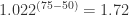 ). An increase of 25% in the percentage of cows dry-treated increases the risk of disease by about 72% (i.e. 1.72 times). Tiestall barns and other barn types both have lower risks of Nocardia mastitis than freestall barns.
