Second part on logistic regression (first one here).
We used in the previous post a likelihood ratio test to compare a full and null model. The same can be done to compare a full and nested model to test the contribution of any subset of parameters:
mod1.nest <- glm(casecont ~ dcpct, family = binomial("logit"),
+             data = nocardia)
lr.mod1.nest <- -(deviance(mod1.nest) / 2)
(lr <- 2 * (lr.mod1 - lr.mod1.nest))
[1] 30.16203
1 - pchisq(lr, 2)
[1] 2.820974e-07
### or, more straightforward, using anova to compare the 2 models:
anova(mod1, mod1.nest, test = "Chisq")
Analysis of Deviance Table

Model 1: casecont ~ dcpct + dneo + dclox
Model 2: casecont ~ dcpct
  Resid. Df Resid. Dev Df Deviance  Pr(>Chi)
1       104     107.99
2       106     138.15 -2  -30.162 2.821e-07 ***
---
Signif. codes:  0 ‘***’ 0.001 ‘**’ 0.01 ‘*’ 0.05 ‘.’ 0.1 ‘ ’ 1
Interpretation of coefficients
### example 16.2
nocardia$dbarn <- as.factor(nocardia$dbarn)
mod2 <- glm(casecont ~ dcpct + dneo + dclox + dbarn,
+               family = binomial("logit"), data = nocardia)
(mod2.sum <- summary(mod2))

Call:
glm(formula = casecont ~ dcpct + dneo + dclox + dbarn, family = binomial("logit"),
    data = nocardia)

Deviance Residuals:
    Min       1Q   Median       3Q      Max
-1.6949  -0.7853   0.1021   0.7692   2.6801

Coefficients:
               Estimate Std. Error z value Pr(>|z|)
(Intercept)   -2.445696   0.854328  -2.863  0.00420 **
dcpct          0.021604   0.007657   2.821  0.00478 **
dneoYes        2.685280   0.677273   3.965 7.34e-05 ***
dcloxYes      -1.235266   0.580976  -2.126  0.03349 *
dbarntiestall -1.333732   0.631925  -2.111  0.03481 *
dbarnother    -0.218350   1.154293  -0.189  0.84996
---
Signif. codes:  0 ‘***’ 0.001 ‘**’ 0.01 ‘*’ 0.05 ‘.’ 0.1 ‘ ’ 1

(Dispersion parameter for binomial family taken to be 1)

    Null deviance: 149.72  on 107  degrees of freedom
Residual deviance: 102.32  on 102  degrees of freedom
AIC: 114.32

Number of Fisher Scoring iterations: 5

cbind(exp(coef(mod2)), exp(confint(mod2)))
Waiting for profiling to be done...
                               2.5 %     97.5 %
(Intercept)    0.08666577 0.01410982  0.4105607
dcpct          1.02183934 1.00731552  1.0383941
dneoYes       14.66230075 4.33039752 64.5869271
dcloxYes       0.29075729 0.08934565  0.8889877
dbarntiestall  0.26349219 0.06729031  0.8468235
dbarnother     0.80384385 0.08168466  8.2851189
Note: Dohoo do not report the profile likelihood-based confidence interval on page 404. As said in the previous post, the profile likelihood-based CI is preferable due to the Hauck-Donner effect (overestimation of the SE).
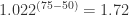
Using neomycin in the herd increases the log odds of Nocardia mastitis by 2.7 units (or using neomycin increases the odds 14.7 times). Since Nocardia mastitis is a rare condition, we can interpret the odds ratio as a risk ratio (RR) and say neomycin increases the risk of Nocardia mastitis by 15 times. Changing the percentage of dry cows treated from 50 to 75% increases the log odds of disease by 
The significance of the main effects can be tested with:
drop1(mod2, test = "Chisq")
Single term deletions

Model:
casecont ~ dcpct + dneo + dclox + as.factor(dbarn)
                 Df Deviance    AIC     LRT  Pr(>Chi)
<none>                102.32 114.32
dcpct             1   111.36 121.36  9.0388  0.002643 **
dneo              1   123.91 133.91 21.5939 3.369e-06 ***
dclox             1   107.02 117.02  4.7021  0.030126 *
as.factor(dbarn)  2   107.99 115.99  5.6707  0.058697 .
---
Signif. codes:  0 ‘***’ 0.001 ‘**’ 0.01 ‘*’ 0.05 ‘.’ 0.1 ‘ ’ 1
The drop1 function tests each predictor relative to the full model.
Presenting effects of factors on the probability scale
Usually we think about the probability of disease rather than the odds, and the probability of disease is not linearly related to the factor of interest. A unit increase in the factor does not increase the probability of disease by a fixed amount. It depends on the level of the factor and the levels of other factors in the model.
mod1 <- glm(casecont ~ dcpct + dneo + dclox, family = binomial("logit"),
+             data = nocardia)
nocardia$neo.pred <- predict(mod1, type = "response", se.fit = FALSE)
library(ggplot2)
ggplot(nocardia, aes(x = dcpct, y = neo.pred, group = dneo,
+                      colour = factor(dneo))) +
+   stat_smooth(method = "glm", family = "binomial", se = FALSE) +
+   labs(colour = "Neomycin", x = "Percent of cows dry treated",
+        y = "Probability of Nocardia")

Next: evaluating logistic regression models.
