We continue on the linear regression chapter the book Veterinary Epidemiologic Research.
Using same data as last post and running example 14.12:
tmp <- tempfile()
download.file("http://ic.upei.ca/ver/sites/ic.upei.ca.ver/files/ver2_data_R.zip", tmp) # fetch the file into the temporary file
load(unz(tmp, "ver2_data_R/daisy2.rdata")) # extract the target file from the temporary file
unlink(tmp) # remove the temporary file

### some data management
daisy2 <- daisy2[daisy2$h7 == 1, ] # we only use a subset of the data
library(Hmisc)
daisy2 <- upData(daisy2, labels = c(region = 'Region', herd = 'Herd number',
                           cow = 'Cow number',
                           study_lact = 'Study lactation number',
                           herd_size = 'Herd size',
                           mwp = "Minimum wait period for herd",
                           parity = 'Lactation number',
                  milk120 = 'Milk volume in first 120 days of lactation',
                           calv_dt = 'Calving date',
                           cf = 'Calving to first service interval',
                           fs = 'Conception at first service',
                           cc = 'Calving to conception interval',
                           wpc = 'Interval from wait period to conception',
                           spc = 'Services to conception', twin = 'Twins born',
                           dyst = 'Dystocia at calving',
                           rp = 'Retained placenta at calving',
                           vag_disch = 'Vaginal discharge observed',
                           h7 = 'Indicator for 7 herd subset'),
                 levels = list(fs = list('No' = 0, 'Yes' = 1),
                   twin = list('No' = 0, 'Yes' = 1),
                   dyst = list('No' = 0, 'Yes' = 1),
                   rp = list('No' = 0, 'Yes' = 1),
                   vag_disch = list('No' = 0, 'Yes' = 1)),
                 units = c(milk120 = "litres"))

library(lubridate)
daisy2$date <- as.character(daisy2$calv_dt)
daisy2$date <- ymd(daisy2$date)
daisy2$mth <- month(daisy2$date)
# calving in automn or not:
daisy2$aut_calv <- with(daisy2, ifelse(mth %in% c(9:12), "fall", "other"))
# centering variables:
daisy2$hs100 <- daisy2$herd_size / 100
daisy2$hs100_ct <- daisy2$hs100 - mean(daisy2$hs100)
daisy2$hs100_ctsq <- daisy2$hs100_ct^2
daisy2$parity_sc <- daisy2$parity - mean(daisy2$parity)

daisy3 <- daisy2[complete.cases(daisy2), ] # df with only complete cases

lm.wpc <- lm(wpc ~ aut_calv + hs100_ct + hs100_ctsq + parity_sc + twin +
+              dyst + rp + vag_disch + rp*vag_disch, data = daisy3)
(lm.wpc.sum <- summary(lm.wpc))

Call:
lm(formula = wpc ~ aut_calv + hs100_ct + hs100_ctsq + parity_sc +
    twin + dyst + rp + vag_disch + rp * vag_disch, data = daisy3)

Residuals:
Interval from wait period to conception
   Min     1Q Median     3Q    Max
-76.40 -35.23 -15.22  22.64 210.63

Coefficients:
                   Estimate Std. Error t value Pr(>|t|)
(Intercept)         66.9831     2.4970  26.825  < 2e-16 ***
aut_calvother       -6.1336     2.6420  -2.322 0.020385 *
hs100_ct            21.8485     2.2546   9.690  < 2e-16 ***
hs100_ctsq          11.7763     3.1952   3.686 0.000236 ***
parity_sc            1.1421     0.8727   1.309 0.190848
twinYes             19.7621     9.8677   2.003 0.045387 *
dystYes             11.0347     5.5386   1.992 0.046515 *
rpYes                7.1111     4.8654   1.462 0.144067
vag_dischYes         2.0977     7.2588   0.289 0.772629
rpYes:vag_dischYes  19.9543    12.7239   1.568 0.117031
---
Signif. codes:  0 ‘***’ 0.001 ‘**’ 0.01 ‘*’ 0.05 ‘.’ 0.1 ‘ ’ 1

Residual standard error: 50 on 1515 degrees of freedom
Multiple R-squared: 0.07355,	Adjusted R-squared: 0.06805
F-statistic: 13.36 on 9 and 1515 DF,  p-value: < 2.2e-16
Now we can create some plots to assess the major assumptions of linear regression. First, let’s have a look at homoscedasticity, or constant variance of residuals. You can run a statistical test, the Cook-Weisberg test (or Breusch-Pagan test), available in libraries car and lmtest:
library(car)
ncvTest(lm.wpc)
Non-constant Variance Score Test
Variance formula: ~ fitted.values
Chisquare = 23.08052    Df = 1     p = 1.553565e-06

library(lmtest)
bptest(lm.wpc)

	studentized Breusch-Pagan test

data:  lm.wpc
BP = 24.3082, df = 9, p-value = 0.00384
Both tests are significant indicating the presence of heteroscedasticity but they are slightly different. Quoting John Fox from this post: “bp.test() performs the same score test as ncvTest(), except that the default alternative hypothesis is different — in bp.test() the error variance is a function of a linear combination of the regressors and in ncvTest() the error variance is a function of the fitted values (i.e., a *particular* linear combination of regressors). Testing against the fitted values with 1 df will have greater power if this is the real pattern of heteroscedasticity”.
But the evaluation of linear model assumptions relies more often on graphical methods. You can use the 6 diagnostic plots readily available after fitting your model, or try it with ggplot2 using the fortify() method which allow combining a model with its data (“the model fortifies the data, and the data fortifies the model”):
plot.lm(lm.wpc, which = 1) # diag plot in base stats package
library(ggplot2)
ggplot(lm.wpc, aes(.fitted, .resid)) +
   geom_hline(yintercept = 0) +
   geom_point() +
   geom_smooth(se = FALSE)

We can check the normality of the residuals by a statistical test, the Shapiro-Wilk test, and a normal probability plot (Q-Q plot):
shapiro.test(resid(lm.wpc))

	Shapiro-Wilk normality test

data:  resid(lm.wpc)
W = 0.8817, p-value < 2.2e-16

ggplot(lm.wpc, aes(sample = .stdresid)) +
   stat_qq() +
   geom_abline()

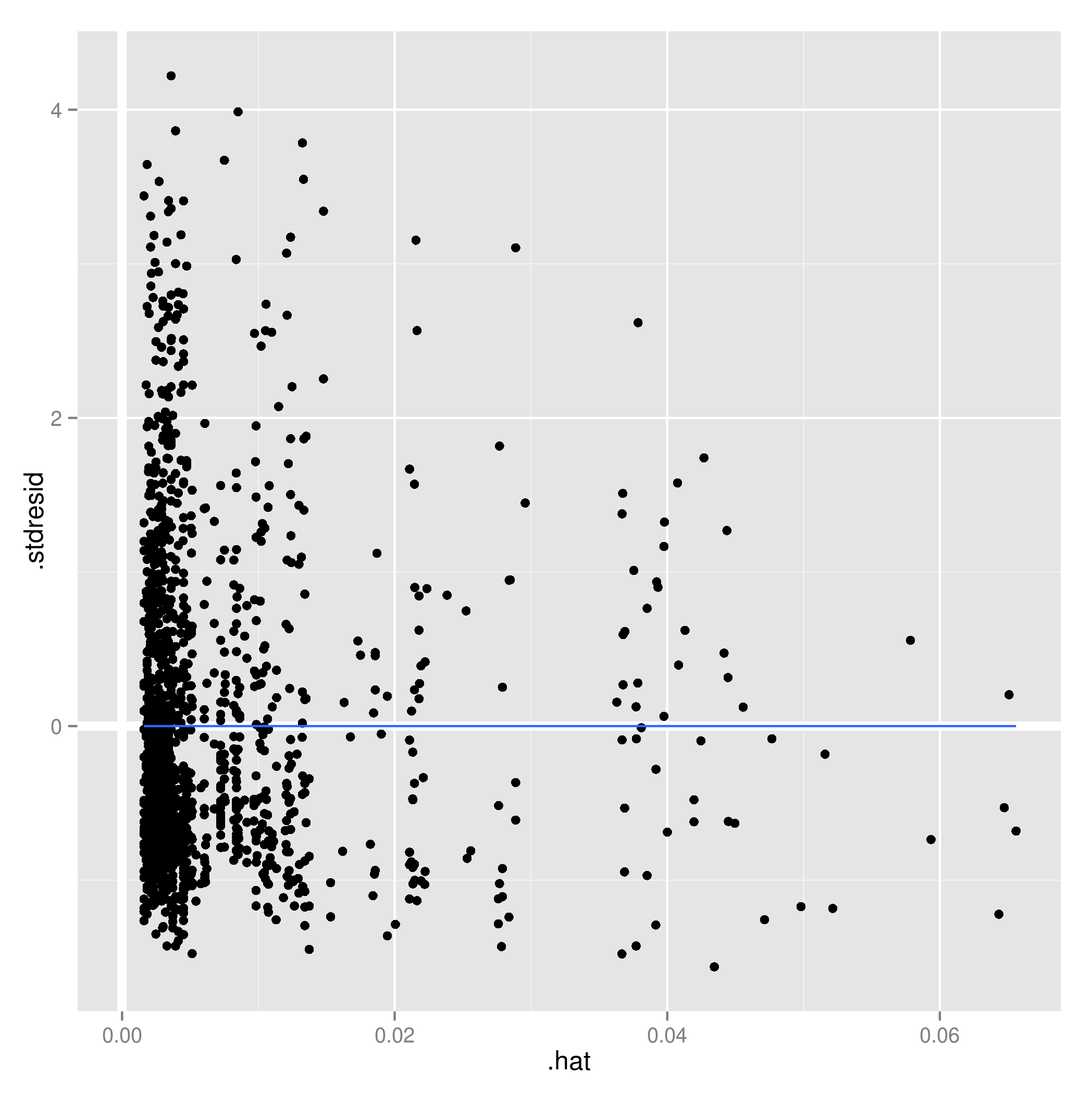
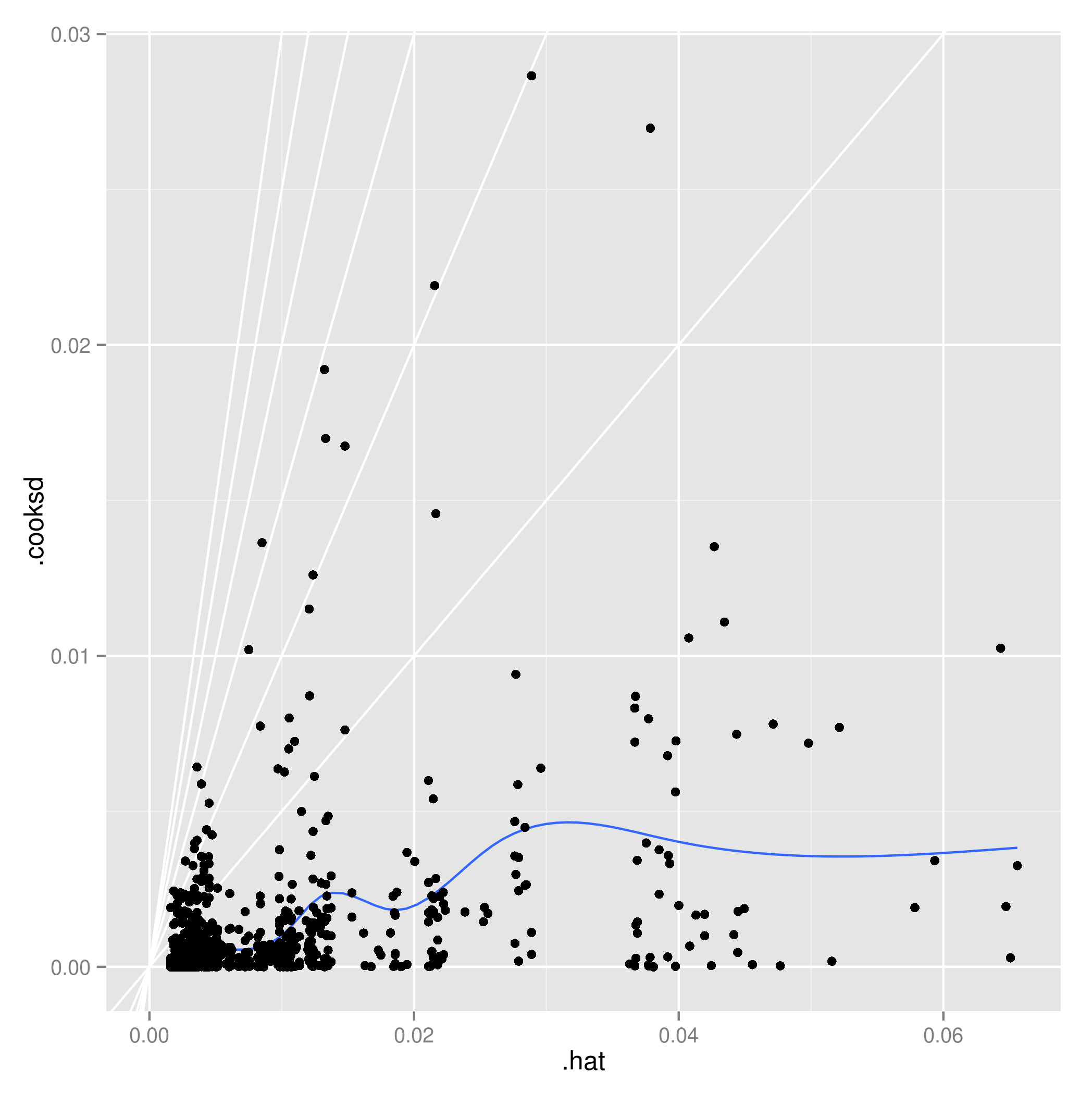
Other diagnostic plots: Scale-Location plot of sqrt(|residuals|) against fitted values, Cook’s distance plot, Residuals vs. leverages, Cook’s distances vs. leverages:
## Scale-Location plot of sqrt(|residuals|) against fitted values (which = 3)
ggplot(lm.wpc, aes(.fitted, abs(.stdresid))) +
       geom_point() +
       geom_smooth(se = FALSE) +
       scale_y_sqrt()

# Cook's distance plot (which = 4)
ggplot(lm.wpc, aes(seq_along(.cooksd), .cooksd)) +
  geom_bar(stat = "identity")

# Residuals vs. leverages (which = 5)
ggplot(lm.wpc, aes(.hat, .stdresid)) +
  geom_vline(size = 2, colour = "white", xintercept = 0) +
  geom_hline(size = 2, colour = "white", yintercept = 0) +
  geom_point() +
  geom_smooth(se = FALSE)

# Cook's distances  vs leverages/(1-leverages) (which = 6)
ggplot(lm.wpc, aes(.hat, .cooksd)) +
  geom_vline(colour = NA) +
  geom_abline(slope = seq(0, 3, by = 0.5), colour = "white") +
  geom_smooth(se = FALSE) +
  geom_point()


You could also check the linearity of the predictor-outcome association by plotting the residuals against each of the continuous predictor variables, for example here centered herd size:
ggplot(lm.wpc, aes(hs100_ct, .resid)) +
  geom_point() +
  geom_smooth(method = "loess", se = FALSE)

Log Transformation
Let’s do a log transformation (with a simpler model) and back-transform the coefficients:
daisy3$milk120.sq <- daisy3$milk120^2
lm.wpc2 <- lm(wpc ~ vag_disch + milk120 + milk120.sq, data = daisy3)
lm.lwpc <- lm(log(wpc) ~ vag_disch + milk120 + milk120.sq, data = daisy3)
(lm.lwpc.sum <- summary(lm.lwpc))

Call:
lm(formula = log(wpc) ~ vag_disch + milk120 + milk120.sq, data = daisy3)

Residuals:
Interval from wait period to conception
    Min      1Q  Median      3Q     Max
-3.9229 -0.5554  0.0231  0.5794  1.7245

Coefficients:
               Estimate Std. Error t value Pr(>|t|)
(Intercept)   4.765e+00  3.140e-01  15.175   <2e-16 ***
vag_dischYes  1.477e-01  8.761e-02   1.686   0.0921 .
milk120      -4.664e-04  1.951e-04  -2.390   0.0170 *
milk120.sq    6.399e-08  2.965e-08   2.159   0.0310 *
---
Signif. codes:  0 ‘***’ 0.001 ‘**’ 0.01 ‘*’ 0.05 ‘.’ 0.1 ‘ ’ 1

Residual standard error: 0.7615 on 1521 degrees of freedom
Multiple R-squared: 0.006997,	Adjusted R-squared: 0.005039
F-statistic: 3.573 on 3 and 1521 DF,  p-value: 0.01356

(ci.lwpc <- confint(lm.lwpc)) # confidence intervals
                     2.5 %        97.5 %
(Intercept)   4.149060e+00  5.380862e+00
vag_dischYes -2.416148e-02  3.195190e-01
milk120      -8.491117e-04 -8.367357e-05
milk120.sq    5.844004e-09  1.221453e-07
exp(lm.lwpc$coefficients[2])
vag_dischYes
     1.15914
exp(ci.lwpc[2, 1])
[1] 0.9761281
exp(ci.lwpc[2, 2])
[1] 1.376465
The trick to get the confidence interval is to get it on the transformed scale and then going back to the original scale. The most difficult part is in interpreting the results. A proprty of the logarithm is that “the difference between logs is the log of the ratio”. So the mean waiting period length difference between cows with and without vaginal discharge is 0.15 on a log scale, or exp(0.15) = 1.15 times longer for cows with vaginal discharge. Better maybe, express as ratios: the ratio of waiting periods from cows with vaginal discharge or no discharge is 1.15 (95% CI: 0.98 to 1.38). Note that the back-transformation of the confidence interval is not symmetric anymore.
So for your model 


Thank you for this great posting! What I am missing is a short explanation on how to interprete the plots. While, for instance, the results of the Cook-Weisberg-test are easy to read, what are the desired patterns of a plot? How should plots look like so one can say that all covariates fulfil the assumptions? It would be great if you could deliver some notes on that in addition…
Thanks, but the objective of these posts are only to re-do the examples from Ian Dohoo’s book with R, not specifically to go through the theory. But I’ll keep it in mind for a future post!
great series of posts!
you should replace
daisy2$parity_sc <- daisy2$parity – mean(daisy2$parity)
with
daisy2$parity_sc <- as.numeric(daisy2$parity) – mean(as.numeric(daisy2$parity))
because it gives
Warning messages:
1: In mean.default(daisy2$parity) :
argument is not numeric or logical: returning NA
2: In Ops.factor(daisy2$parity, mean(daisy2$parity)) :
– not meaningful for factors
Hi Burfee,
If you use the code above as is, with the dataset downloaded from the Web, you don’t need to switch back parity to a numeric variable. If you use the dairy dataset from the previous post, you’re right you have to change back that variable from factor to numeric. The parity variable (and a few others) were made as factors in the previous post (see lapply function at the top of the post).
Cheers!